A Biologically Interpretable Graph Convolutional Network to Link Genetic Risk Pathways and Imaging Phenotypes of Disease, ICLR 2022 poster [Paper]

Summary

• Similar trend to biologically-informed deep learning, using GAT with pooling
• Outperform PRS (but only one case). It should be vailidated by other disease or other population
• Interpretation is quite good

Introduction

Imaging-genetics is an emerging field that tries to merge these complementary viewpoints

Data-driven imaging-genetics methods can be grouped into four categories. 1) The first category uses sparse multivariate regression to predict one or more imaging features based on a linear combination of SNPs (Wang et al., 2012; Liu et al., 2014).

2) The second category uses representation learning (Pearlson et al., 2015; Hu et al., 2018) to maximally align the data distributions of the two modalities.

3) The third category relies on generative models (Batmanghelich et al., 2016; Ghosal et al., 2019) to fuse imaging and genetics data with subject diagnosis.

4) The fourth category for imaging-genetics uses deep learning to link the multiple viewpoints (Srinivasagopalan et al., 2019; Zeng et al., 2018; Eraslan et al., 2019; Shen & Thompson, 2020).

Most works (and almost all imaging-genetics analyses) require a drastically reduced set of genetic features to ensure model stability (Bhattacharjee et al., 2012). In terms of scale, a raw dataset of 100K SNPs is reduced to 1K SNPs In contrast, neuropsychiatric disorders are polygenetic, meaning that they are influenced by numerous genetic variants interacting across many biological pathways. The GWAS sub-selection step effectively removes the downstream information about these interactions (Horv´ath et al., 2015). The works of (van Hilten et al., 2020; Gaudelet et al., 2020) have used this information to design a sparse artificial neural network that aggregates genetic risk according to these pathways in order to predict a phenotypic variable.

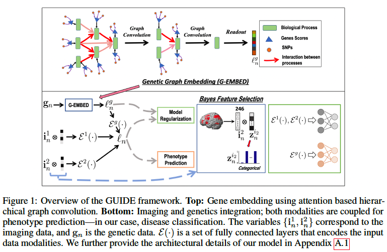
In this paper, they introduce an interpretable Genetics and mUltimodal Imaging based DEep neural network (GUIDE), for whole-brain and whole-genome analysis. They use hierarchical graph convolutions that mimic an ontology based network of biological processes (Mi et al., 2013). They use pooling to capture the information flow through the graph and graph attention to learn the salient edges, thus identifying key pathways associated with the disorder. On the imaging front, they use an encoder coupled with Bayesian feature selection to learn multivariate importance scores. The latent embeddings learned by our genetics graph convolutions and imaging encoder are combined for disease prediction

Method

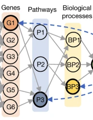
SNPs -> Genes -> BPs -> single vector representation

For subject n,

• imaging features: i_n¹∈ℜ^M₁×1, i_n²∈ℜ^M₂×1
• gene scores: g_n ∈ ℜ^G×1 (G is # of genes)
  The gene scores g_n are obtained by grouping the original SNPs according to the nearest gene and aggregating the associated genetic risk weighted by GWAS effect size. (Like PRS)
• phenotype y_n ∈ {0,1}

Genetic graph embedding (Gene -> BP)

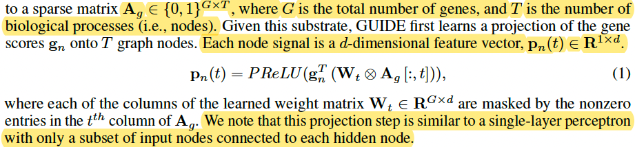
Like a projection from gene to BP by d sparse neural network

(From Haitham A. Elmarakeby et al.)
This projection step is similar to a single-layer perceptron with only a subset of input nodes connected to each hidden node.

Graph attention and hierarchical pooling
Use a graph convolution to mimic the flow of information through the hierarchy of biological processes (GAT).
Use hierarchical pooling to coarsen the graph.
Thus, remove the lowest (leaf) layer from the graph at each stage l and continue this process until we reach the root nodes. The genetic embedding ℓ_n^g &in;ℜ^D</sub>×1 is obtained by concatenating the signals from each root node.

Bayesian feature selection
Skip

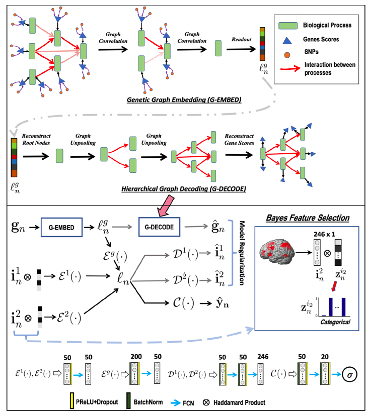
Multimodel fusion and model regularization

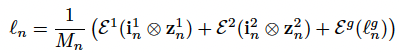
ε(·) is fully connected nn

They introduce three regularizers to stabilize the model. 1) The genetic regularizer reconstructs the gene scores by performing a hierarchical graph decoding (G-DECODE) on ℓ_n^g. 2) Likewise, the imaging regularizer decodes the original feature vectors from ℓ_n via the artificial neural networks D^m(·). 3) Skip (regularizer regrading bayesian feature selection)

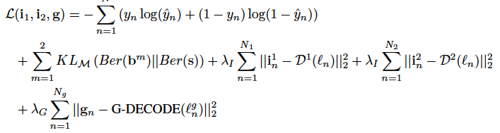
The first two terms of Eq. (7) correspond to the classification task and the feature sparsity penalty, which are empirical translations of Eq. (4). The final three terms are the reconstruction losses, which act as regularizers to ensure that the latent embedding is capturing the original data distribution.

Training Strategy
Note, they can accommodate missing data during training by updating individual branches of the network based on which modalities are present. In this way, GUIDE can maximally use and learn from incomplete data.

As described in Section 4, experimental dataset consists of 1848 subjects with only genetics data and an additional 208 subjects with both imaging and genetics data. Given the high genetics dimensionality, they pretrain the G-EMBED and G-DECODE branches and classifier of GUIDE using the 1848 genetics-only subjects. These 1848 subjects are divided into a training and validation set, the latter of which is used for early stopping. We use the pretrained model to warm start GUIDE framework and perform 10-fold nested CV over the 208 imaging-genetics cohort.

Implementation details
Use first five layers of the gene ontology to construct G-ENCODE. In total, this network encompasses 13595 biological processes organized from 2836 leaf nodes to 3276 root nodes.
Fix the signal dimensionality at d = 2 (initial dim) for the gene embedding and d_l = 5 (hidden dim) for the subsequent graph convolution and deconvolution operations based on the genetics-only subjects.
initial learning rate of 0.0002 and decay of 0.7 every 50 epochs.

Baseline comparison methods

Evaluation strategy
(1) Influence of the Ontology-Based Hierarchy
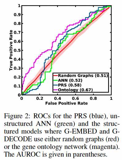
To test it, they compare their gene ontology network to random networks and to an unstructured model.

• random network: randomly permute edges between the parents and children nodes, and between the genetic inputs and nodes g_n
• unstructured: a fully-connected ANN

They compare the deep learning models with the gold-standard Polygenetic Risk Score (PRS) for schizophrenia developed by the PGC consortium.

(2) Classification Performance
repeated 10-fold cross validation (CV) on the imaging 208 genetics subjects to quantify the performance. trained using 8 folds, and the remaining two folds are reserved for validation and testing. Further use DeLong tests to compare statistical difference in AUROC between GUIDE and the baselines.

(3) Reproducibility of Feature Importance Maps
They extract the the top features of learned top-K features of b_m during each training fold of our repeated 10-fold CV setup and encode this information as a binary indicator vector, where the entry ‘1’ indicates that the feature is among the top-K.

Compare the BFS features with Kernel SHAP. \

• To quantify predictive performance, they mask their test data from each fold using the BFS and K-SHAP indicator vectors and send it through GUIDE for patient versus control classification
• To quantify the reproducibility of the top-K features, we calculate the pairwise cosine similarity between all the binary vectors across the folds as identified by either BFS or K-SHAP.

(4) Discovering of Biological Pathways
The attention layer of G-ENCODE provides a subject specific measure of “information flow” through the network
The importance of edges along these paths are used in a logistic regression framework to predict the subject class label. (?)
They then perform a likelihood ratio test and obtain a p-value (FDR corrected) for each path in terms of patient/control differentiation.
For robustness, we repeat this experiment 10 times using subsets of 90% of our total dataset 1848 + 208 subjects and select pathways that achieve p < 0.05 in at least 7 of the 10 subsets.

Results

Data and preprocessing
Illumina Bead Chipset including 510K/ 610K/660K/2.5M is used for genotyping. Quality control and imputation were performed using PLINK and IMPUTE2. The resulting 102K linkage disequilibrium independent (r2<0.1) indexed SNPs are grouped to the nearest gene (within 50kb basepairs)
The 13,908 dimensional input genes cores are computed as weighted average of the SNPs using GWAS effect size.
1848 subjects (792 schizophrenia, 1056 control) with just SNP data
208 subjects with imaging and SNP data

(1) Benefit of the Gene Ontology Network
First train just the genetics branch and classifier for all three deep networks (unstructured, random graphs, ontology) using the 1848 genetics-only subjects and test them on the SNP data from the other 208 subjects.

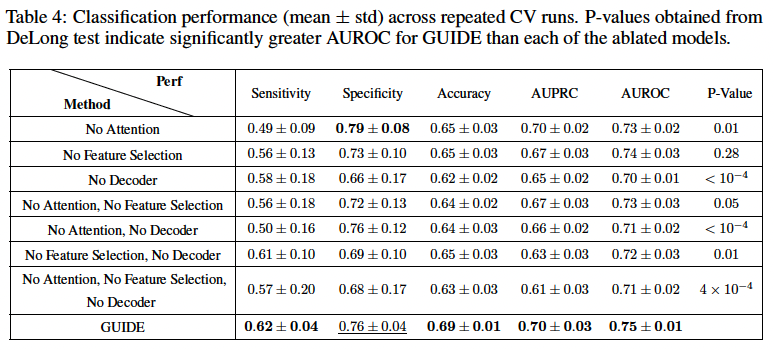
(2) Classification performance
10-fold CV testing performance of all the methods on the multimodal imaging-genetics dataset; repeat the CV procedure 10 times to obtain standard deviations for each metric

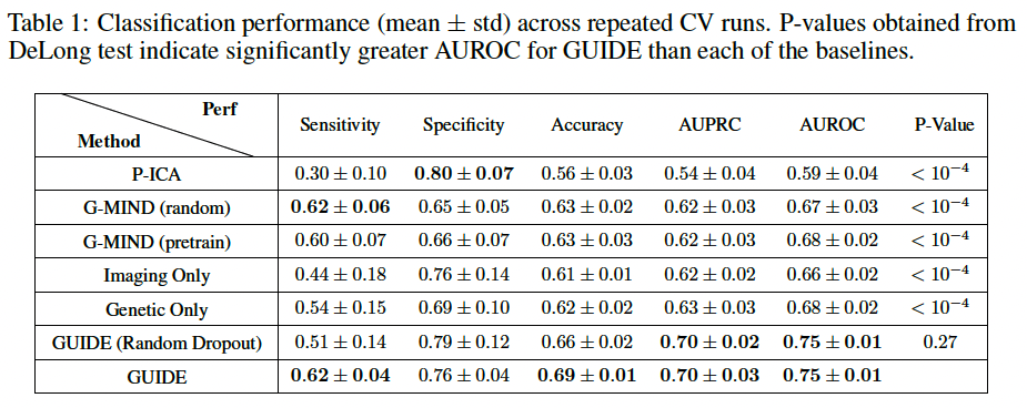
They also evaluate replacing the GUIDE BFS layer with random dropout. While the quantitative performance is similar, the feature reproduciblity is much higher with BFS.

(3) Reproducibility of BFS Features

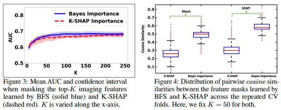
Fig. 3 illustrates the classification AUC when the input features are masked according to the top-K importance scores learned by the BFS (solid blue) and K-SHAP (dashed red) procedures.
Fig. 4 illustrates the distribution of cosine similarities between the masked feature vectors learned by BFS and K-SHAP for K=50

(4) Genetic Pathways
From 14881 “biological pathways” between the leaf and root nodes, identify 152 pathways with p < 0.05 after FDR correction that appear in at least 7 of the 10 random training datasets. Use the tf-idf (Beel et al., 2016) information retrieval scheme to extract keywords in the pathways; then embed them in a two-dimensional space using t-SNE and apply a k-means clustering algorithm.

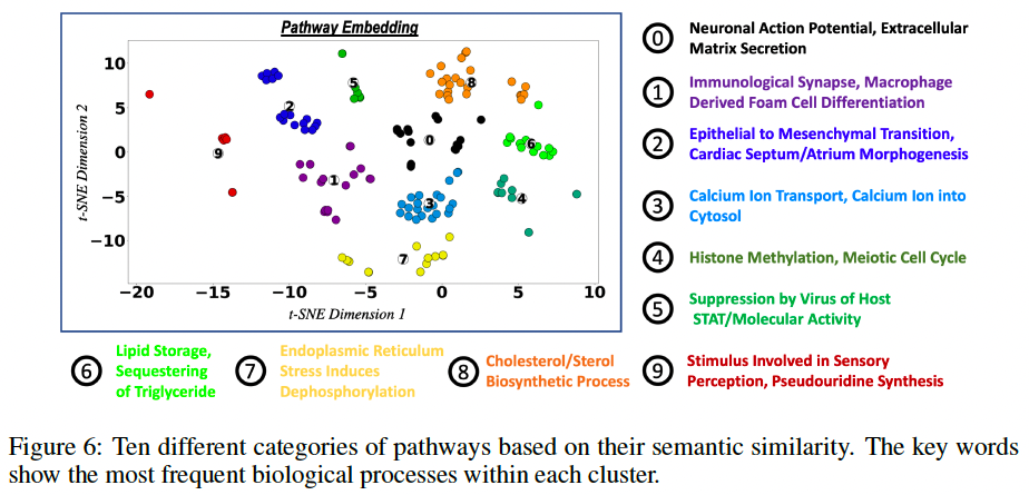
Fig. 6 shows the clusters along with the most frequent keywords within each cluster. cluster these pathways into 10 categories based on their semantic similarity

Ablation study

Question

• how to identify important pathway? The description is unclear.